Complete Introduction to Capacitors
November 13, 2023
Complete Introduction to Capacitors
This tutorial is a deep dive into comprehensive knowledge of capacitors and will guide you through everything you need to know about them, all in one place.Capacitors are one of the most fundamental components we use for influencing the behavior of electric circuits. Capacitors can be used for storing energy, conducting alternating current (AC), and blocking or separating direct current (DC). There are many types of capacitors out there that are differentiated by the materials used in construction, each providing certain benefit features which make it better for some applications. Understanding basic capacitor construction and how different materials can affect their characteristics will give you a help with choosing the proper capacitor for your projects. They can be divided into two basic groups: electrostatic capacitors and electrolytic capacitors.
What is Electrostatic Capacitor?
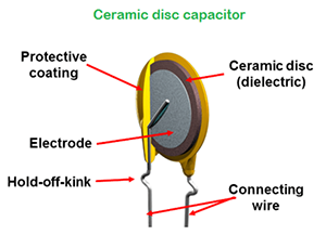
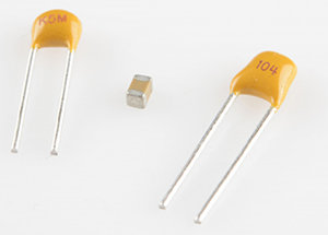
Electrostatic capacitors have symmetrical non-polar terminals. Material such as plastic film and ceramic are used as the dielectric, while electrodes can be made from a variety of metals. Since these parts are not polarized, they can generally be inserted into a circuit without regard to which points the terminals are connected.The electrostatic capacitor most commonly seen around us is Ceramic Capacitor, the name comes from the material from which their dielectric is made. Ceramic capacitors have a small value in both of physical size and capacitance. It's hard to find a ceramic capacitor much larger than 10μF. Ceramic capacitors are a near-ideal capacitor that they have low ESR and leakage current. ESR is short for Equivalent Series Resistance. But their small capacitance can be limiting; electrostatic capacitors are generally used for small or precise capacitance values that they are widely used for high-frequency coupling and decoupling circuits. The construction of ceramic capacitor is as shown as below,
What is Electrolytic Capacitor?
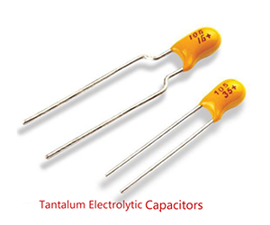
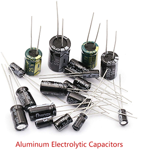
Electrolytic capacitors are different from electrostatic capacitors, they have asymmetric and polarized terminals. Electrolytic capacitors utilize an electrolyte which may maintain the dielectric layer and also create the negative terminal, or cathode. Metal foil or powders, such as aluminum and tantalum, are used to form the positive connection(anode). The dielectric layer is created by forming a thin oxide on the metal anode. For example, in aluminum electrolytic capacitors, the anode is aluminum, the dielectric is aluminum oxide, and the liquid electrolyte is also the cathode. Since these capacitors are polarized, care must be taken to ensure they are designed and inserted correctly into circuits, for aluminum electrolytic capacitors, the leg of the anode might be slightly longer as another indication. If voltage is applied in reverse on an electrolytic capacitor, a pop and bursting open may happen, the capacitor will be damaged permanently.
Compared to the equally popular electrostatic capacitors , electrolytic capacitors generally have large capacitance in the range of 1μF to 1mF, they are well suited to high voltage applications as they have relatively high maximum rating in voltage. The prominent drawback of electrolytic capacitors is leakage that allow small amounts of current (on the level of nano amperes, or nA) to run through the dielectric from one terminal to the other. This makes electrolytic capacitors less-than-ideal for energy storage.
Structure of Capacitors
Even different kinds of capacitors are made from different kinds of materials to suit related applications down to ground but all the capacitors are formed with the same basic structure.
As Fig. (0.0.1) shown, two parallel metal electrode plates are separated by a non-conductive material. The non-conductive material can be known as dielectric, examples of dielectric material are glass, air, paper, plastic, ceramic and so on. Dielectric is an insulating material sits between the two metal electrode plates that to make sure they do not touch with each other and prevent large amount of electricity from flowing one side to the other directly.
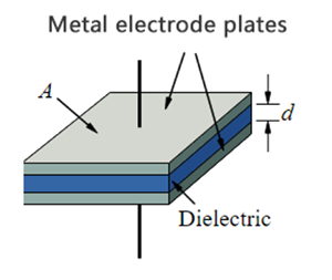 Figure (0.0.1)
Capacitance is the parameter that indicating the ability of a capacitor to store the electric charge. Denoted by C, the unit of capacitance is F (farad), in honor of the English physicist Michael Faraday. The capacitance of a capacitor can be presented with the following equation:
(2.0.0)
or
(2.0.1)
or
(2.0.2)
Where ε is absolute permittivity, often simply called permittivity
εr is the dielectric's relative permittivity
εo is vacuum permittivity
A is the surface area of each plate
d is the distance between the plates
We can learn from Eq. (2.0.0) that the following three factors determine the value of the capacitance:
- The overlapping surface area of the plates, the more area, the greater the capacitance
- The distance between the plates, the more distance, the smaller the capacitance
- The permittivity of the material, the higher the permittivity, the greater the capacitance
Typically, capacitors have values in pF (picofarad) to microfarad (μF), the reason why we seldom see a capacitor marked as F (farad) is that because farad is a high value. To convert μF to nF or pF or to a wide range of other units and vice versa, we need to use the Electric Capacitance Unit Converter.
- 1 mF (milli farad) = 10-3 F = 103 μF = 106 nF = 109pF
- 1 μF (microfarad) =10-6 F = 10-3mF = 103 nF = 106 pF
- 1 nF (nano farad) = 10-9 F = 10-3μF = 10-6mF = 103 pF
- 1 pF (picofarad) = 10-12 F = 10-3nF = 10-6μF = 10-9mF
How Capacitor Works
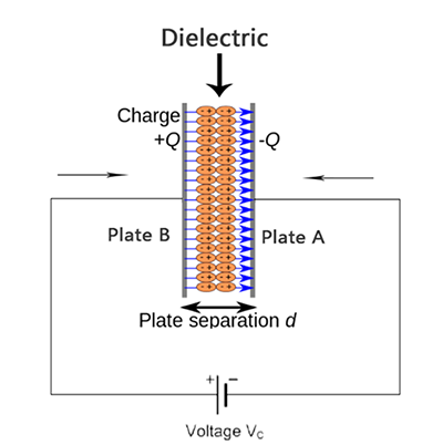 Figure (0.0.2)
Charging a Capacitor
In Fig. (0.0.2), when a voltage source is applied to a capacitor, electrons move from cathode of the voltage source to Plate A, as there is an insulating dielectric region sitting between Plate A and Plate B and the electrons could not flow through to reach plate B that, the electrons are sucked into plate A. In our physical world, two electrons will tend to repel each other because both have a negative electrical charge. The large amounts of negative charges on plate A push away like charges on plate B, making plate B positively charged. The electrons that are pushed away from plate B to the anode of voltage source that, generating a current from anode of voltage source to plate B, if we put a LED between anode of voltage source and plate B, the LED will be lighted up for a while and then going out. Some beginners may say that current is the flow of electrons. No! Current is the flow of positive charged particles that the moving direction is opposite to electrons. Current behaves as positive charges carries current flow or conventional current flow. In our convention, current is an electric stream flows from the positive electrode to the negative, but what actually happens it is that the electrons flow out of the negative terminal, through the circuit and into the positive terminal of the power source. It is important to realize that the difference between conventional current flow and electron flow in no way effects any real-world behavior or computational results. In general, analyzing an electrical circuit yields results that are independent of the assumed direction of current flow. Conventional current flow is the standard that most all of the world follows.
At some point the capacitor plates will be so full of charges that they just can't accept any more. There are enough negative charges on plate A that they can repel any others that try to join, no more charge will be increased. The positive charges on plate B and negative charges on plate A that create an electric field, this field stores energy and produces a mechanical force between the plates. The present amount of charges stored, represented by Q (The unit of Q is c, coulomb), is directly proportional to the applied voltage V, the equation is,
Q = CV (2.0.3)
From Eq. (2.0.3) we get that, capacitance is the ratio of the charge on one plate of a capacitor to the voltage difference between the two plates, 1 farad = 1coulomb/volt, or 1F = 1c/v. BUT please note that the capacitance does not depend on Q or V, it just only depends on the three factors mentioned in the part of Eq. (2.0.0). That means the Q and V cannot affect its capacitance once the capacitor has been made.
Since Current is the rate of flow of charges, a current of 1 A (ampere) means that 1 c (coulomb) of charges flows through a point in a circuit per second. The equations is,
Q = I.t (2.0.4)
We take the derivative of Eq. (2.0.4) to obtain the amount of charges in a period of time, we get,
or
(2.0.5)
From Eq. (2.0.3) and Eq. (2.0.5) we can obtain the current of the charging capacitor,
(2.0.6)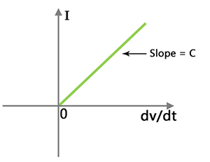 Figure (0.0.3)
Fig. (0.0.3) is the Current-voltage/time relationship of a capacitor without resistor connected in series
dV/dt is the derivative of the voltage with respect to time. In other words, it's the change in voltage (delta V, or ΔV) divided by the change in time (delta t, or Δt), or the rate at which the voltage changes over time. The big takeaway from Eq. (2.0.6) is that if voltage is steady, the dV is zero, which means current is also zero. This is why current cannot flow through a capacitor holding a steady, DC (direct current) voltage. However, the applied voltage could not be infinitely increasing, when the voltage is continuously increased, the dielectric material will at some point not withstand the electric field between the electrodes, causing the dielectric to break down.
Charging a Capacitor with Series Resistor
When connect a resistor in series with the capacitor like Fig. (0.0.4), the things may become a little bit complicated that we cannot analyze the circuit just like the process mentioned above. We have to consider how the new adding resistor will affect the charging time of the capacitor and what would happen if we increase or decrease the value of the resistor. This is where the Time Constant comes into play.
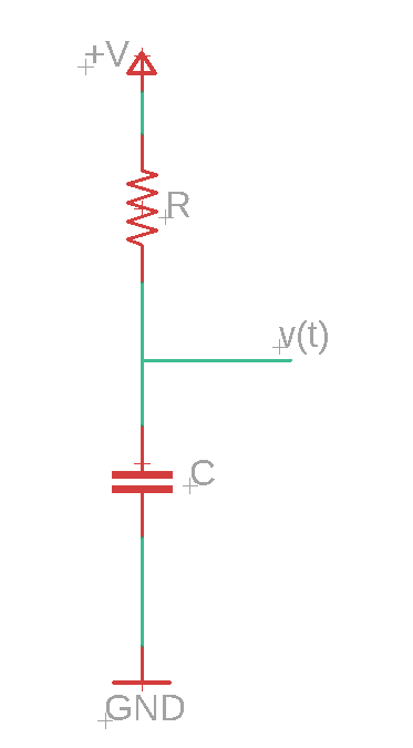 Figure (0.0.4)
What is RC Time Constant?
RC time constant is the time required to charge the capacitor from the voltage of zero to 63.2% of the value of DC power source of the circuit or to discharge the capacitor through the same resistor to approximately 36.8% of its initial charged voltage. Time constant is also called Tau, symbolized as τ. RC constant often come out to be in the hundredths of a second or millisecond range. Time constant is measured by the Eq. (2.0.7)
(2.0.7)Where R is the resistance of the series resistor (in ohms), C is the capacitance of the capacitor (in farads), fc is the Cutoff Frequency of the RC circuit, from Eq. (2.0.7) we get the cutoff frequency of the RC circuit is,
(2.0.8)Why is the Time Constant represented by RC?
Some beginners just wonder why does the Time Constant is defined as the product of the series resistance and capacitance. Here I will expound the proving process in mathematical equations.
In Fig. (0.0.4), when voltage V is applied at time t =0. The current starts flowing through the resistor R and the capacitor starts charging. As a result of this the voltage v(t) on the capacitor C starts increasing. The charge q(t) on the capacitor also starts rising. The amount of the charge q(t) at any time t is,
(2.0.9)Differentiating this equation with respect to time, we get,
(2.1.0)is the rate of the change of charge, i.e. current i(t) through the series circuit at time t, from Eq. (2.1.0), we get,
(2.1.1)from Kirchoff's law, we get,
(2.1.2)Where v(t) is the voltage across the capacitor at time t
Combining Eq. (2.1.1) and Eq. (2.1.2), we get,
or
(2.1.3)
Solving the Eq. (2.1.3), we get,
 (2.1.4)
 Where K in Eq. (2.1.4) is a constant of integration
When at t =0, v(t) = 0,
(2.1.5)Combining Eq. (2.1.4) and Eq. (2.1.5), we get,
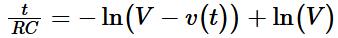
or
(2.1.6)
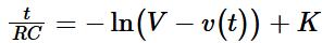
Expressing the Eq. (2.1.6) in exponent form, we get,
or
(2.1.7)
When t = RC, we get,
(2.1.8)So, from the Eq. (2.1.8), we can learn that why the time constant is equal to RC. The character e is a famous irrational number which is one of the most important numbers in mathematics, its value is approximately equal to 2.72. Thus, 1-e-1 = 1 – 1/2.72 ≈ 1 – 0.368 = 63.2%.
RC charging circuit curve can be drawn as Fig. (0.0.5)
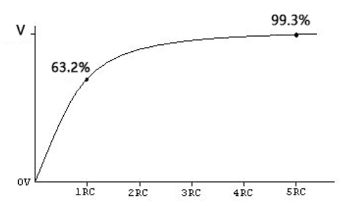 Figure (0.0.5)
The RC charging table as shown in Fig. (0.0.6)
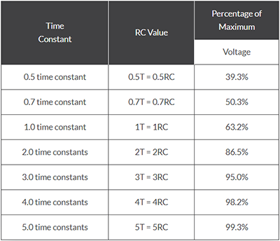 Figure (0.0.6)
The things are quite clear that from t =0 to 1RC constant the charging curve is steeper as the charging rate is fastest, when at the time of 1RC the voltage cross the capacitor reach 63.2% of the power source voltage. From 1RC to 5RC the charging curve tappers off as the capacitor takes on additional charge at a slower rate. When at time of 5RC the capacitor voltage can reach 99.3% of the power voltage. When the time after 5RC, the RC circuit step into Steady State Period, no more charge can be added to the capacitor. The maximum applied voltage across the capacitor is 99.3% of the power source voltage, NOT 100%. The reason why the capacitor in reality never becomes 100% fully charged due to the energy stored in the electric field the capacitor.
Discharging a Capacitor
Suppose we have a capacitor, C charged up until it reaches an amount of time equal to 5 times of RC constants and remains fully charged. And then adjust the circuit that looks like Fig. (0.0.7),
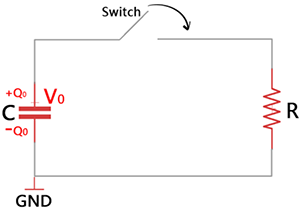 Figure (0.0.7)
In Fig. (0.0.7), the capacitor initially has +Q0 and -Q0 on the capacitor plates, the initial potential difference is V0. In RC discharging circuit, the time constant is the time required to discharge the capacitor through the same resistor to approximately 36.8% of its initial charged voltage V0. That means after one RC constant time the voltage across the capacitor has dropped by 63.2% of its initial charged value. When the switch is closed, there is a current, I(t) flow through the resistor that serves to reduce the amount of charge on the capacitor that reduce the voltage across the capacitor; the relationship of charge and voltage is,
(2.1.9)From Kirchhoff’s Law, we get,
(2.2.0)Since we know,
(2.2.1)Combining Eq. (2.2.0) and Eq. (2.2.1), we get,
or
(2.2.2)
To solve the differential equation Eq. (2.2.2), we need to intergrade both sides and get,
(2.2.3)from Eq. (2.2.3), we get,
(2.2.4)Taking the exponential of both sides of Eq. (2.2.4), we get,
(2.2.4a)Combining Eq. (2.1.9) and Eq. (2.2.4a), we get,
(2.2.5)Where V0 is the initial voltage on the capacitor when the time, t=0.
From Eq. (2.2.5), we can learn that why the time constant is equal to RC. The number e is a famous irrational number which is one of the most important numbers in mathematics, its value is approximately equal to 2.72. Thus, e-1 = 1/2.72 ≈ 0.368 = 36.8%.That means when t=RC, V(t) = 36.8%V0.
The discharging curve can be drawn as Fig. (0.0.8)
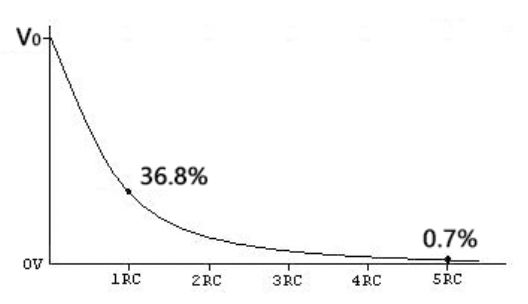 Figure (0.0.8)
The discharging table is showing as Fig. (0.0.9),
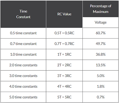 Figure (0.0.9)
From Fig. (0.0.8), we can see that the discharging curve for a RC discharging circuit is exponential. After on constant time, the capacitor discharge down to about 36.8% of its initial voltage, V0. And then after five RC time constants a capacitor is considered to be fully discharged.
Conclusion: In an RC circuit, the time constant is the product of the Resistance, R and the Capacitance, C that is a measure of how quickly it either charge or discharge. Where, R is in Ω and C in Farads.
Charging and Discharging Curves
Through the detailed analysis of charging and discharging, we can use the following figure (Fig.0.09-a) for time sequence analysis. The first waveform is a pulse signal with a width of 6RC. The middle waveform is the voltage change trajectory of the capacitor charging and discharging. The bottom waveform is the current change trajectory of the capacitor charging and discharging. These three waveforms all share the same time sequence:
 Fig.0.09-a
It can be simplified as shown below:
 Fig.0.09-b
During the charging process, current (i) flows into the capacitor, causing its plates to start holding electrostatic charge. This charging process is not instantaneous or linear, because when the capacitor plates are uncharged, the intensity of the charging current reaches its maximum value, and it decreases exponentially over time until the capacitor is fully charged.
The charging current of a capacitor can be defined as: . Once the capacitor is "fully charged", it will prevent more electrons from flowing to its plates because they have become saturated. Therefore, we see that the charging curve of the capacitor is an increasing curve with decreasing curvature, and the charging current curve accompanying this charging process is a decreasing curve with decreasing curvature. The charging current of the capacitor is the derivative of the charging voltage, and the same applies to discharge.
Capacitive Reactance in AC Signals
Like resistance, reactance is also measured in ohms (Ω), but it's denoted by the symbol X to distinguish it from pure resistance values (R). Reactance has two types: inductive reactance (XL) caused by inductors and capacitive reactance (XC) caused by capacitors. Inductive reactance opposes changes in current, while capacitive reactance opposes changes in voltage in an AC circuit.
For capacitors in an AC circuit, capacitive reactance is represented by the symbol XC. So, we can actually say that Capacitive Reactance is a capacitive resistance value that changes with frequency. Furthermore, capacitive reactance depends on the capacitance of the capacitor measured in farads and the frequency of the AC waveform. The formula used to define capacitive reactance is as follows:
Where the unit of F is hertz, and the unit of C is farads. 2πƒ can also be collectively referred to as the Greek letter Omega, ω, which represents angular frequency.
From the above capacitive reactance formula, it can be seen that if either the frequency or the capacitance is increased, the overall capacitive reactance will decrease. As the frequency approaches infinity, the capacitive reactance of the capacitor will decrease to zero, acting like a perfect conductor.
Phase Shift in Capacitor Charging and Discharging
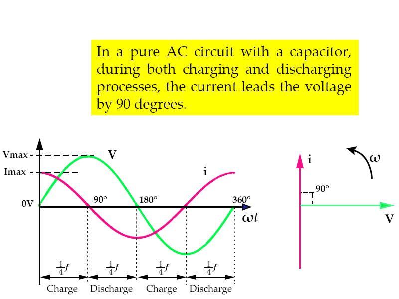 Fig.0.09-c
- At 0°, the rate of change of the power supply voltage increases in the positive direction, resulting in the maximum charging current at that moment.
- At 90°, the power supply voltage reaches its maximum and temporarily remains constant, at which point the current is 0.
- At 180°, the slope of the voltage is negative, and the capacitor discharges in the negative direction. At 180° along the line, the rate of voltage change reaches its maximum again.
From the waveform in Fig.0.09-c above, we can see that the current leads the voltage by cycle or 90°. So, we can say that in a pure capacitive circuit (an ideal state with a capacitive reactance of 0), the AC voltage lags the current by 90°.
RC Differentiator (High Pass Filter)
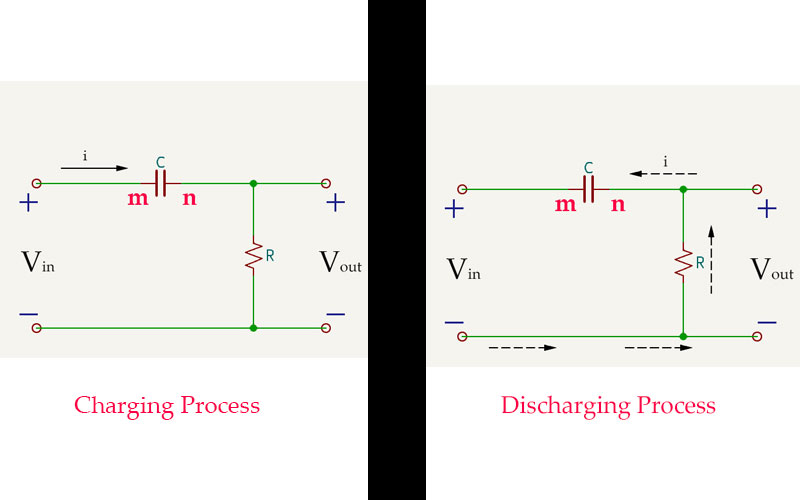 Fig.0.09-d
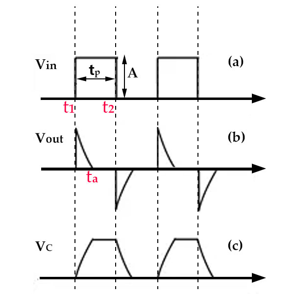 Fig.0.09-e
When there is no input signal, Vin=VC=Vout=0.
Now we apply a pulse signal as shown in Fig. 0.09-e to the input terminal.
-
When t = t1:
At t1, the voltage at the m-terminal of capacitor, C suddenly rises to the value labeled as ‘A’ in Fig. 0.09-e (a). Due to the characteristic of capacitors resisting abrupt voltage changes across their terminals, a voltage of value ‘A’ is induced at the n-terminal of the capacitor. This maintains a voltage difference of 0 between the 'm' and 'n' of the capacitor (the duration of this induced voltage at the 'n' is extremely short and depends on the resistance, R connected in series with capacitor (C)). The corresponding waveform for this process is shown in Fig. 0.09-e (b). At t1, Vout suddenly rises to its maximum value, and the voltage across the capacitor, C becomes (A) , i.e. VC=A. -
When t1<t<t2:
During the time from t1 to t2, the voltage becomes a constant value, equivalent to a direct current voltage, and the capacitor is no longer in a charging state. Due to the capacitor's ability to pass alternating current and block direct current, the voltage induced at the n-end of the capacitor will discharge through R, and the voltage will exponentially decrease. At t=ta, it drops to 0 (since tp>>RC, at this time the signal pulse is still in a high voltage state, but the capacitor is already fully charged. For the capacitor, only when the voltage changes within Δt time can current be generated, and a constant value voltage cannot generate current, so the current flowing through R at this time is 0, and the voltage across R - that is, the output voltage is 0). -
When t=t2:
When it reaches the moment t2, due to Vin suddenly dropping to 0V, the capacitor, in order to maintain the voltage at both ends m and n, will induce a negative voltage at the n-end, with a value of -A. This induced voltage is instantaneous. At this time, the capacitor will discharge through the resistor R. Since the negative pole of the signal is 0V, and the n-end of the capacitor is -A, the direction of the current is opposite to the direction during charging, as indicated by the dashed arrow in the Discharging Process diagram in Fig.0.09-d. The waveform corresponding to this process is the waveform below the horizontal axis in Fig.0.09-e(b).
For example, when the resistance R in Fig.0.09-d is 20KΩ, the capacitance C is 100pF, the amplitude of the input signal is 5V, and the pulse width is 50μs, the changes of Vin and Vout are shown in Fig.0.09-f below:
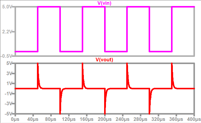 Fig.0.09-f
It should be noted that in the differential circuit, the time constant τ (the product of R and C) needs to be much smaller than the pulse width tp of the input signal (generally τ < 0.2tp). τ = RC<<tp, where tp is the width of the rectangular pulse. The smaller τ is, the faster the charging and discharging speed of the capacitor, and the sharper the output pulse, and vice versa. Because the smaller the value of τ, the shorter the time required for the capacitor to be fully charged and discharged, the easier it is for a spike to occur in a shorter period of time, this is also the reason why RC<<tp is required.
Based on this condition, we can approximate the capacitor voltage VC(t) as the input signal voltage Vin(t):
As , so, ; As , so, .
the capacitive resistance
Summing up the above two formulas, we can get . According to Ohm's law, therefore, VC(t) >> Vout(t), VC(t) ≈ Vin(t)
Assuming the initial voltage state Vc(t0) = 0V, the current after the capacitor is charged can be calculated by the following formula:
As Q=C.V, Q= I.t, so, C.V = I.t, so,
Combining the relationship between the voltage and current of the capacitor, it can be concluded that the output of the circuit is the derivative of the input voltage:
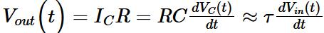
Vout is the voltage across the resistor R.
For example, when the resistor R in Fig.0.09-d is 20KΩ and the capacitor C is 2.5 nF, the input is still the aforementioned pulse signal. At this time, τ = RC = tp, which no longer satisfies the prerequisite condition of RC<<tp. The voltage changes of Vin and Vout are shown in the Fig.0.09-g below. At this point, the output of Vout is no longer a sharp spike pulse.
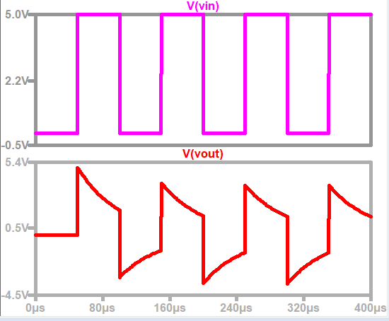 Fig.0.09-g
High Pass Filter
The RC Differentiator circuit can also be used as a High Pass Filter, allowing only alternating current signals above a specific frequency to pass through. For example, when the resistor R is 2KΩ and the capacitor C is 1μF, the cutoff frequency is calculated to be approximately 79.16Hz according to the formula . The AC signal analysis is shown in the Fig.0.09-h below (the solid line represents the amplitude of the signal, while the dashed line indicates the phase shift of the signal, lagging or leading the input signal).
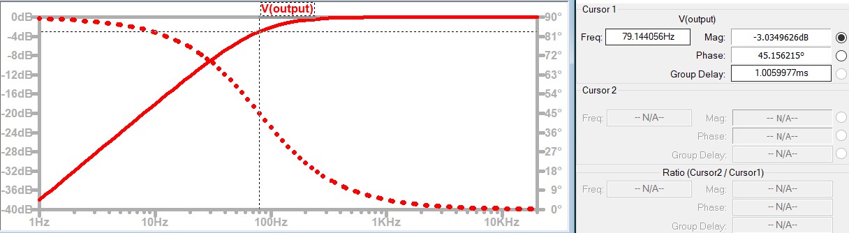 Fig.0.09-h
From the above figure Fig.0.09-h, it can be seen that when the signal frequency is 79.16Hz, the output signal attenuation is approximately -3dB. From this, the following graph of the relationship between Frequency and dB can be drawn:
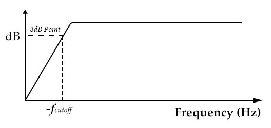 Fig.0.09-i
Signals with a frequency lower than Fc cannot pass through this RC circuit. Only when the signal frequency is higher than Fc can it pass through with low or even no attenuation.
RC Integrator (Low Pass Filter)
By swapping the positions of the resistor and capacitor in the RC differentiator circuit, we obtain the integrator circuit as shown in Fig.0.09-j. This circuit is relatively easy to understand. It utilizes the principle that the voltage across the capacitor cannot change abruptly. When Vin = A, the capacitor C is charged and Vout gradually increases. When Vin becomes 0, the capacitor C discharges through the resistor R and Vout gradually decreases, and this process repeats. The integrator circuit can be used to convert a square wave into a sawtooth wave output. The condition for this to hold is the time constant τ, where RC >> tp. The charging and discharging speed of the capacitor is far slower than the speed of pulse changes, this allows the initial part of charging curve of the capacitor to be applied to both ends of the capacitor. The ends of the capacitor serve as the output, so the integrator circuit can convert a square wave into a sawtooth wave or a triangular wave. If RC >> tp is not satisfied, the voltage C will saturate, and it will not achieve the purpose of converting a square wave into a triangular wave or a sawtooth wave.
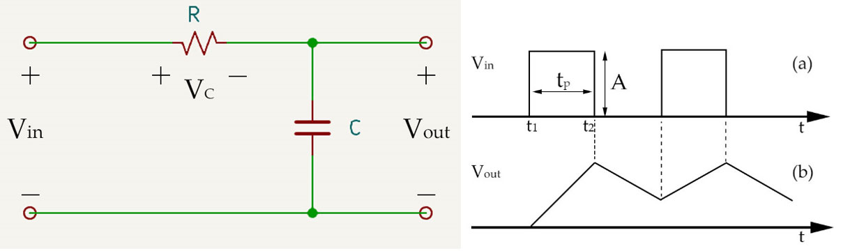 Fig.0.09-j
As Q=C.V, so, ;
As Q=I.t, so,
The output is directly taken from the voltage across the capacitor, therefore the output is the integral of the input voltage:
 Vout is equal to the voltage across the capacitor C.
Low Pass Filter
The RC integrator circuit can also be used as a Low Pass Filter, allowing only alternating current signals below a specific frequency to pass through. For example, when the resistor R is 1KΩ and the capacitor C is 100nF, the cutoff frequency is calculated to be approximately 1592Hz according to the formula .

The AC signal analysis is shown in the figure below (the solid line represents the amplitude of the signal, while the dashed line indicates the phase shift of the signal, lagging or leading the input signal):
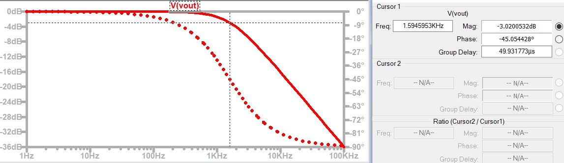 Fig.0.09-k
From the above figure Fig.0.09-k, it can be seen that when the signal frequency is 1592Hz, the output signal attenuation is approximately -3dB. From this, the following graph of the relationship between Frequency and dB can be drawn:
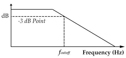 Fig.0.09-m
Signals with a frequency higher than FC cannot pass through this RC circuit. Only when the signal frequency is lower than Fc can it pass through with low or even no attenuation.
Capacitors in Series
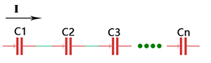 Figure (0.1.0)
For N capacitors connected in series, the current, I flow through each capacitor is the Same,i.e. I=I1 = I2 = I3 =…= In. From charge Q(t) = I.dt, we get,
Q1 = Q2 = Q3 =…= Qn = Q. (2.2.6)
That means, capacitors connected together in series must have the same charge.
By Kirchhoff's Voltage Law, the total voltage applied to the series circuit, Vt is the sum of the voltage cross each capacitor, we get,
Vt = V1 + V2 + V3 +…+Vn (2.2.7)
As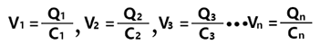 (2.2.8)
If in the series capacitors circuit, the equivalent capacitance is Ct, Combining Eq. (2.2.6) and Eq. (2.2.7) and Eq. (2.2.8),we get,
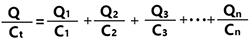
or
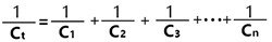 (2.2.9)
As we can see from Eq. (2.2.9), the total capacitance (or equivalent capacitance) of N capacitors in series is the reciprocal of the sum of the reciprocals of the individual capacitances.
Capacitors in Parallel
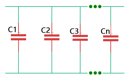 Figure (0.1.1)
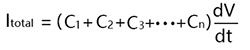
In Fig. (0.1.1), for N capacitors connected in parallel as shown in Fig. (0.1.1), the total current Itotal is the sum of the currents flow each capacitor. The voltage across each capacitor is the same.
From Q = CV and Q=I.t we get,
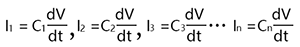 (2.3.0)
As we know,
Itotal = I1 + I2 + I3 +…+In (2.3.1)
Combining Eq. (2.3.0) and Eq. (2.3.1), we get,
 (2.3.2)
Let us replace these parallel capacitors by a single equivalent capacitor Ctotal, we get,
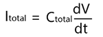 (2.3.3)
From Eq. (2.3.2) and Eq. (2.3.3), we get,
 (2.3.4)
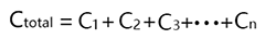
As we can see from Eq. (2.3.4), the total capacitance (or equivalent capacitance) of N capacitors in parallel is the sum of the individual capacitances.
Capacitor in Rectifier Circuit
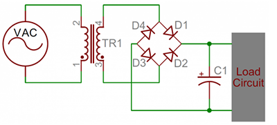 Figure (0.1.2)
Capacitor in rectifier circuit is one of the most common applications that uses both of capacitor charging and discharging features to smooth the output. We typically use the capacitors with sufficient high capacitance in smoothing circuits, such as the electrolytic capacitors. In a Full Wave Rectifier Circuit like Fig. (0.1.2), if without the capacitor, the DC voltage generated by the rectifier is consisted of half sine waves, like Fig. (0.1.3) shows, the voltage range is between zero and √2 times of RMS(root-mean-square) voltage that is not a smooth output voltage.
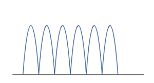 Figure (0.1.3)
By adding a parallel capacitor to the rectifier, the output can be turned into a near-level DC voltage like the red line part in Fig. (0.1.4),
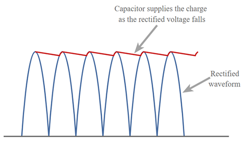 Figure (0.1.4)
The capacitor charges up as the rectified voltage rises. When the rectified voltage falls downward, the capacitor will release current from its stored energy that it'll discharge very slowly, supplying energy to the load. The capacitor shouldn't fully discharge before the input rectified voltage starts to rise again, recharging the capacitor, expressed as the equation like Eq. (2.3.5),
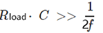 (2.3.5)
- Where Rtotal is resistance of the load circuit
- C is the capacitance of the capacitor in Farads
- f is the input frequency
Eq. (2.3.5) tells that the choice of the capacitance needs to meet the requirement that its time constant RC is very much longer than the time interval between the successive peaks of the rectified waveform (the reciprocal of 2f in full wave rectifier circuit is the period of a wave or time interval of one cycle of the wave).
If in a Half Wave Rectifier Circuit, the equation is,
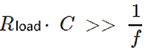 (2.3.6)
The Half Wave Rectifier output voltage is as shown like Fig. (0.1.5)
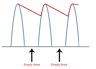 Figure (0.1.5)
Please note that Full Wave Rectifier Circuit is composed of four diodes that to form a Diode Bridge Rectifier while Half Wave Rectifier Circuit is just has one diode like Fig. (0.1.6) shows,
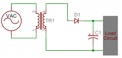 Figure (0.1.6)
Creative Commons tutorials are CC BY-SA 4.0 License